Bước 2: Đánh giá mức độ phân bố chuẩn

Check the normality assumpttion

Cách 1

library(car)
leveneTest(stability ~ diet*time, data = my_data)

Levene's Test for Homogeneity of Variance (center = median)
      Df F value Pr(>F)
group 15  0.7751 0.6936
      32               

From the output above we can see that the p-value is (0.6936) not less than the significance level of 0.05. This means that there is no evidence to suggest that the variance across groups is statistically significantly different. Therefore, we can assume the homogeneity of variances in the different treatment groups.

Tạm dịch: Kết quả cho thấy p-value là 0.6936 lớn hơn 0.05 (giả thuyết cho là có sự phân bố không chuẩn - heterogeneity). Do đó bộ dataset này có sự phân bố chuẩn (homogeneity) trong sự khác biệt giữa các nghiệm thức.

Cách 2

Cần tính anova trước để có data vẽ đồ thị qqplot

# Compute two-way ANOVA test
res.aov2 <- aov(stability ~ diet + time, data = my_data)
# summary(res.aov2)
# anova(res.aov2)

# Compute two-way ANOVA test with interaction effect
res.aov3 <- aov(stability ~ diet + time + diet:time, data = my_data)
# anova(res.aov3)

Vẽ đồ thị

plot(res.aov3, 1) ## Homogeneity of variances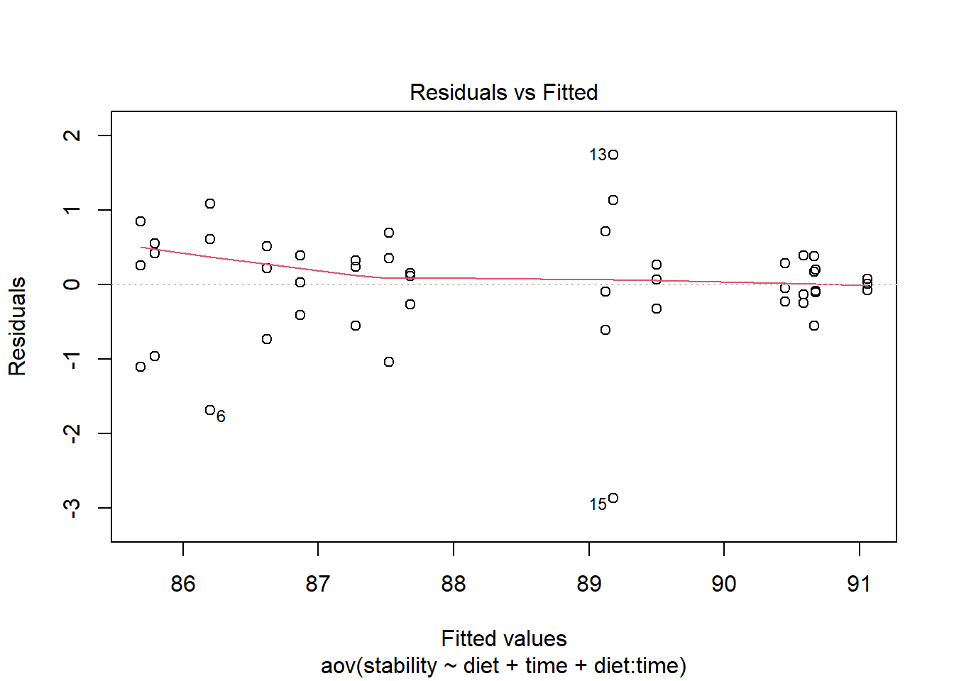

plot(res.aov3, 2) ## Check the normality assumpttion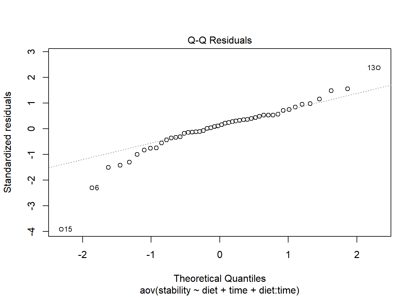

Phát hiện các data point 6, 13, 15 là outlier, có thể loại ra để làm dataset phân bố chuẩn hơn.

Cách 3

# Extract the residuals
aov_residuals <- residuals(object = res.aov3)
# Run Shapiro-Wilk test
shapiro.test(x = aov_residuals) 

    Shapiro-Wilk normality test

data:  aov_residuals
W = 0.91161, p-value = 0.001523

p-value từ test Shapiro-Wilk normality cho thấy nhỏ hơn 0.05 (giả thuyết là phân bố chuẩn), do đó về mặt ý nghĩa thống kê thì bộ dataset này có phân bố chuẩn.